Problem to Solve
Cardiovascular diseases are the leading cause of death worldwide, responsible for the loss of millions of lives each year. This project seeks to detect and predict the determining variables that put us at risk of heart disease, allowing awareness and preventive measures.
The objective is to identify which risk factors (age, blood pressure, cholesterol, lifestyle habits, etc.) have the greatest impact on the probability of developing heart disease, using advanced machine learning techniques to create a robust predictive model.
1. Dataset Information
Two complementary datasets were used that contain information about cardiovascular risk factors and patient health conditions.
Dataset 1: HEARTDISEASE
Tamaño: 3,674 filas × 16 columnas
- sex: Male or female gender
- age: Person's age
- education: Education level
- smokingStatus: Indicates if the person smokes
- cigsPerDay: Number of cigarettes a person smokes per day
- BPMeds: Indicates if the person takes medications (1: yes, 2: no)
- prevalentStroke: Person who had a stroke (1: yes, 0: no)
- prevalentHyp: Person who has hypertension
- diabetes: Person who has diabetes
- totChol: Person's total cholesterol level
- sysBP: Person's systolic blood pressure
- diaBP: Person's diastolic blood pressure
- BMI: Body mass index
- heartRate: Person's resting heart rate
- glucose: Person's blood glucose level
- CHDRisk: Indicates if the person is at risk of heart disease
Dataset 2: HEART_2020_CLEANED
Tamaño: 319,795 filas × 18 columnas
- HeartDisease: Indicates if the person is at risk of heart disease
- BMI: Body mass index
- Smoking: Person who smokes
- AlcoholDrinking: Person who drinks a lot of alcohol (men +14 drinks per week, women +7 drinks per week)
- Stroke: Person who suffered a stroke
- PhysicalHealth: How many of the last 30 days the person exercised
- MentalHealth: How many of the last 30 days the person was not mentally well
- DiffWalking: Person who has difficulty walking or climbing stairs
- Sex: Female or male sex
- AgeCategory: Age category
- Race: Imputed ethnicity value
- Diabetic: Person who was informed they have diabetes
- PhysicalActivity: Adult who reported having performed physical activity during the last 30 days outside their usual work
- GenHealth: Genetics
- SleepTime: Hours of sleep
- Asthma: Person who had asthma
- KidneyDisease: Person who had kidney disease, excluding incontinence
- SkinCancer: Person who had skin cancer
Dataset Examples
Dataset 1 - HEARTDISEASE (Primeras filas)
| sex | age | education | smokingStatus | cigsPerDay | totChol | sysBP | BMI | CHDRisk |
|---|---|---|---|---|---|---|---|---|
| male | 39 | 4 | no | 0 | 195 | 106.0 | 26.97 | no |
| female | 46 | 2 | no | 0 | 250 | 121.0 | 28.73 | no |
Dataset 2 - HEART_2020_CLEANED (Primeras filas)
| HeartDisease | BMI | Smoking | AlcoholDrinking | Stroke | Sex | AgeCategory | PhysicalActivity | GenHealth |
|---|---|---|---|---|---|---|---|---|
| No | 16.60 | Yes | No | No | Female | 55-59 | Yes | Very good |
| No | 20.34 | No | No | Yes | Female | 80 or older | Yes | Very good |
2. Data Wrangling - Dataset Concatenation
Both datasets were concatenated to obtain a more complete unified dataset. This process generates some additional transformations in the data and creates null values in columns that are not common between both datasets.
Unified Dataset
Final size: 323,469 rows × 20 columns
| sex | age | Smoking | diabetes | HeartDisease | BMI | totChol | MentalHealth | AgeCategory | Race |
|---|---|---|---|---|---|---|---|---|---|
| male | 39.0 | no | no | NaN | 26.97 | 195.0 | NaN | NaN | NaN |
| female | 46.0 | no | no | NaN | 28.73 | 250.0 | NaN | NaN | NaN |
Note: NaN values appear in columns that only exist in one of the original datasets.
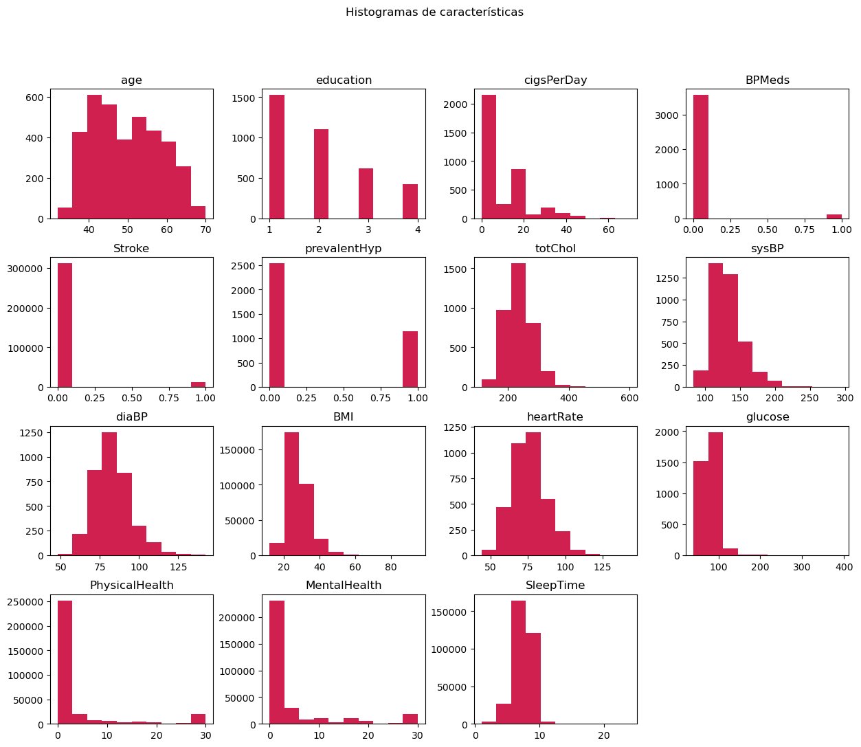
Histogram Analysis
After concatenation, variable histograms were analyzed to understand their distributions and detect possible data problems.
3. Data Processing
3.1 Missing Value Treatment
Different imputation strategies were applied according to variable type and distribution:
Normal Variables
Missing data is replaced with the mean
Non-Normal Variables
Missing data is replaced with the median
Categorical Variables
Missing data is replaced with the mode
3.2 Categorical Variable Encoding
LabelEncoder from scikit-learn was used to convert categorical variables into numeric values.
Before Encoding
| sex | Smoking | diabetes | HeartDisease | AlcoholDrinking | DiffWalking |
|---|---|---|---|---|---|
| male | no | no | no | No | No |
| female | no | no | no | No | No |
| male | yes | no | yes | No | No |
After Encoding
| sex | Smoking | diabetes | HeartDisease | AlcoholDrinking | DiffWalking |
|---|---|---|---|---|---|
| 1 | 0 | 0 | 0 | 0 | 0 |
| 0 | 0 | 0 | 0 | 0 | 0 |
| 1 | 1 | 0 | 1 | 0 | 0 |
3.3 Variable Scaling
Different scaling techniques were applied according to variable distribution:
Standard Scaler
For normal variables. Normalizes data by subtracting the mean and dividing by the standard deviation.
z = (x - μ) / σ
Robust Scaler
For non-normal variables. Uses the median and IQR, being more robust to outliers.
x_scaled = (x - median) / IQR
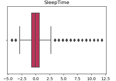
3.4 Outlier Treatment
Atypical values were identified and treated. For normal variables, outliers were replaced with the mean using the Z-Score method.
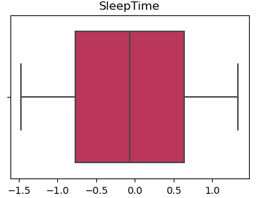
Visual Example - SleepTime Variable
With Outliers
Without Outliers
3.5 Correlation Analysis
The correlation map was analyzed to identify highly correlated variables and eliminate dependencies, avoiding multicollinearity in the models.
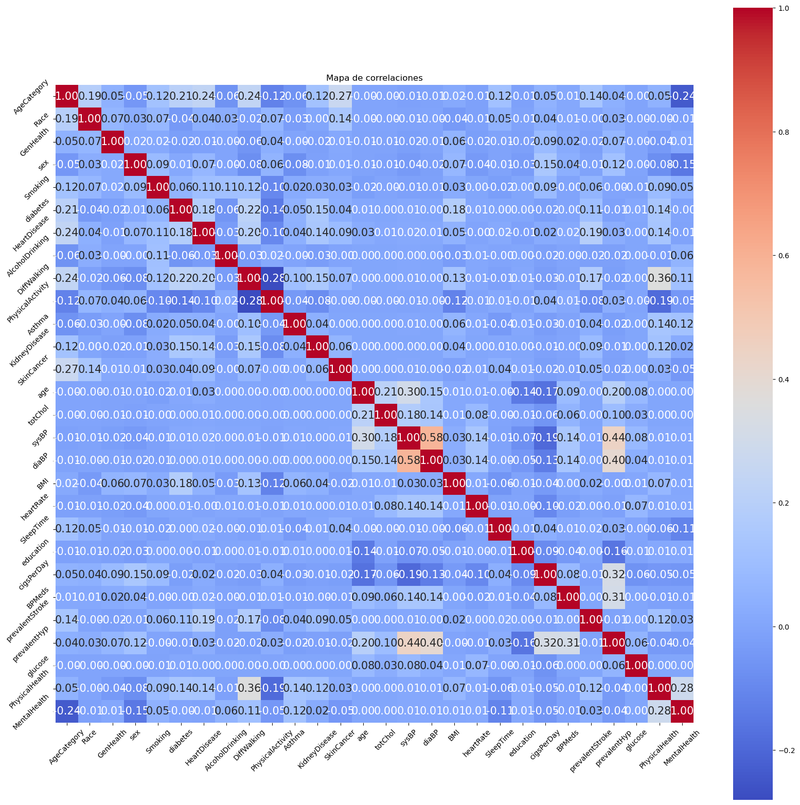
Variables with high correlation were eliminated to avoid the model having redundant information.
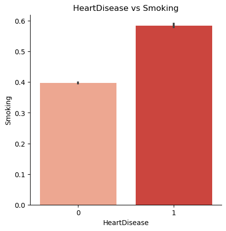
4. Exploratory Data Analysis (EDA)
Exploratory analyses were performed to answer key questions about cardiovascular risk factors.
Does age influence the possibility of developing heart disease?
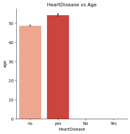
Is a person who smokes more prone to heart disease?
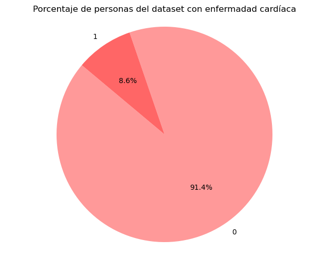
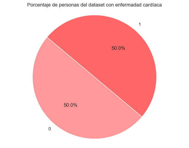
5. Target Variable Balancing
The dataset had a significant imbalance in the target variable. Oversampling technique was applied to create new synthetic samples of the minority class and balance the classes.
Before Balancing
After Balancing
6. Principal Component Analysis (PCA)
PCA (Principal Component Analysis) was applied to reduce dataset dimensionality and eliminate redundancies, maintaining as much information as possible with fewer variables.
What is PCA?
PCA is a dimensionality reduction technique that transforms original variables into principal components (new uncorrelated variables) that capture the maximum possible variance. This helps to:
- Reduce the number of features while maintaining relevant information
- Eliminate redundancies and correlations between variables
- Improve model performance when working with fewer dimensions
Cumulative Explained Variance vs Components
Cumulative explained variance shows how much information from the original data is preserved when using a certain number of principal components. A high value indicates that most of the information is being preserved.
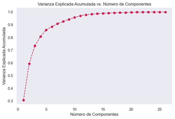
Using the elbow method, it is observed that from component 15 onwards, the variance increases minimally. Therefore, 15 principal components were selected to apply PCA.
7. Model Training
4 different machine learning algorithms were trained and compared, applying advanced validation and optimization techniques for each.
Validation and Optimization Techniques Used
Simple Validation
Division of the dataset into training and test sets to evaluate the model's initial performance.
Cross Validation
Strategy that divides data into k subsets (folds) and trains the model k times, each time using a different fold as the test set. This helps avoid overfitting and provides a more robust performance estimate.
HalvingGridSearchCV
Hyperparameter optimization that combines GridSearch with a "halving" strategy (progressive reduction). It starts by evaluating many parameters with few resources and gradually focuses resources on the most promising combinations, being more efficient than traditional GridSearch.
Model Comparison
| Metric | Decision Tree | Random Forest | Logistic Regression | XGBoost |
|---|---|---|---|---|
| Accuracy | 0.6927 | 0.6933 | 0.7406 | 0.6933 |
| Precision | 0.9101 | 0.9102 | 0.9072 | 0.9102 |
| Recall | 0.6927 | 0.6933 | 0.7406 | 0.6933 |
| F1 Score | 0.7604 | 0.7609 | 0.7960 | 0.7609 |
Conclusion
Comparing all models, it is observed that precision is quite high, reaching 90%, with DecisionTree and XGBoosting even reaching 91%. However, in terms of recall, accuracy, and F1 Score, RandomForest and the Logistic Regression model show more solid metrics. Although the differences are minimal, the final choice leans towards the Logistic Regression model, which slightly outperforms RandomForest in overall performance.